Working With Spreadsheets

Purpose: To get familiar with electronic spreadsheets by using them in some simple applications.

These are pictures of the first spreadsheet we did. We used f(x)=Asin(Bx+C) as our function. We had x start at zero and then go to 10 by 0.1. In the equation, A = amplitude which is 5 in this equation, B = frequency which is 3, and C = phase which is pi/3.
The first picture has the equation shown. In the second picture, we have the numerical value after excel plugged in the numbers.

This is the graph of the plotted points. The x values are that of which we used in excel sheet. It starts at zero and goes to ten by 0.1. The y values are the numerical values we got after excel plugged the numbers into the equation.
The original equation is f(x)=5sin(3x+(pi/3). After doing the best fit quadratic line, out equation comes out to be f(x)=5sin(3x+1.05). This is fairly correct when pi/3 is rounded to two decimal places. We used 1.047198 for pi/3.








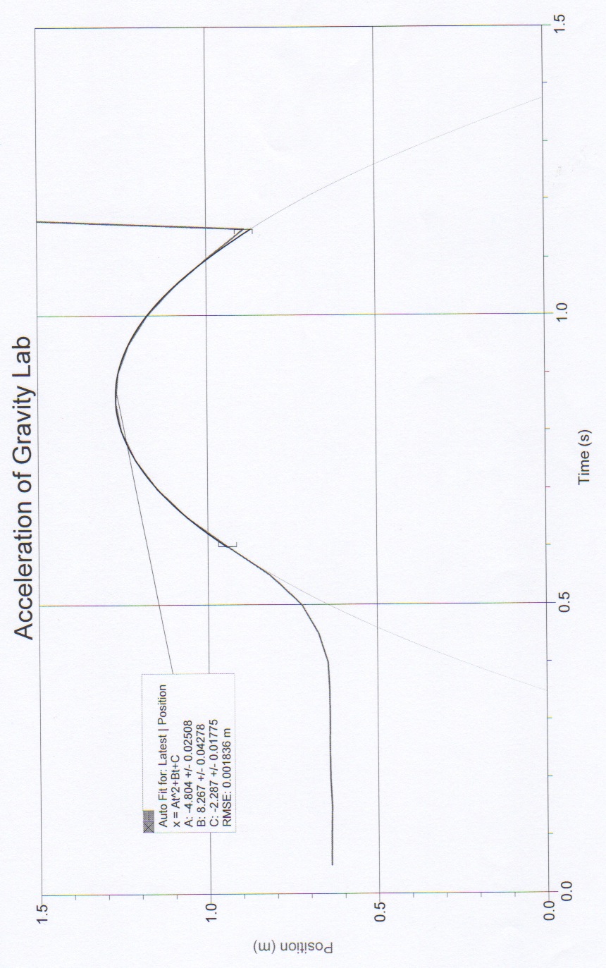
These are the excel spreadsheets from the second equation we did, f(x)=A+Bx+Cx^2. In this equation, A is position (x0) which equals 1000m. B is velocity (v0) which equals 50m/s. Lastly, C is gravity which equals -4.9m/s^2. For the x values, x is represented by delta t which equals 0.2. We interpreted this as the x values start at 0.2 and increase by 0.2 as well. We had it go to ten just like the last equation.
The first spreadsheet shows the equation and the second spreadsheet shows the numerical value after excel plugged the numbers into the equation.

This it the graph that comes from the second equation. The x values are delta t which starts at 0.2 and increase by 0.2. The y values are the numerical values given by plugging the numbers into the equation.
Our original equation was f(x)=1000+50x-4.9x^2. The best fit line we got was f(x)=1000+50x-4.9x^2. The equation is the exact same as the one we used.








Conclusion: This was a good lab to do because we were able to practice or learn how to use excel. It was also good because we could see how the different parts of equations affect the graph. In our group we originally had put acceleration (gravity) as positive 4.9m/s^2. Our graph was completely different from the one that was negative. Our parabola was upside down opening up. That was the only problem we had in this lab. Once we fixed the problem, it all made sense.

Vector Addition of Forces

Purpose: To study vector addition by: 1) Graphical means and 2) Using components. A circular force table is used to check results

Our group started with magnitudes 200cm, 100cm, and 150 cm with degrees of 0, 41, and 132 respectively. This is the graph of the vectors given. Thee scale is 1 cm = 20 g.
Vector D is the resultant force. The angle of vector D and the x-axis is 45 degrees.
This graph also shows the x and y components of each vector.





Vector A) Ax = 200g                                       x = 200+100cos(41)+150cos(132) = 175.1g
                Ay = 0g                                            y = 0+100sin(41)+sin(132) = 177.1g
Vector B) Bx = 100cos(41) = 75.5g
                By = 100sin(41) = 65.6g                 R = 250g at 45 degree
Vector C) Cx = 150cos(132) = -100.4g          Rx = 250cos(45) = 176.8g
                Cy = 150sin(132) = 111.5g             Ry = 250sin(45) = 176.8g
 

This graph is solely the x and y components of each vector. The final vector goes from the tail of the first to the head of the last. That vector is the resultant vector.

These pictures are of the circular force table. Our measurements were correct because the first time we put the weights on at the given angles, it was balanced.

This is the picture from the simulation website. using our vectors, we got the same resultant vector.










Conclusion: In this lab we worked with vectors. We found the resultant vector from three vectors given. With this we found that it is balanced with wights and angles that were given. I learned that vectors are basically trig problems. This problem was fairly simple and we didn't have any errors with calculations. We did calculate our vectors two ways, mathematically and with a graphical approach. In our math we got whole numbers but graphically we got numbers that were decimals but could be rounded to the same numbers as ours. Another source of error comes from using the force table. There could have been friction or it could have been unbalanced (in out favor) which would have thrown off the balance. If out calculations were off and the table wasn't balanced but it said it was is why it would be in our favor.

Acceleration of Gravity on an Inclined Plane

Procedure: 1) To find the acceleration of gravity by studying the motion of a cart on an incline. 2) To gain further experience using the computer for data collection and analysis.


Ramp 1 1.65 degree

This is the first ramp (not drawn to scale). The length of the long leg is 228.2 cm. To find the height (short leg), we took the height from the ramp on either side and then subtracted them. From there we went to find the angle of elevation. We took arc tan(6.2/228.2) and this came out to theta = 1.56 degrees.

Ramp 2 3.6 degree

This is the second ramp (not drawn to scale). This one had larger angle of elevation. We did the same thing to both sides of the ramp to find the height and it came out to be 14.3 cm. Then we took arc tan(14.3/228.2). Theta = 3.6 degrees.

Graph 1

This is the position verses time graph. It is a parabola because the car went up the ramp and then back down. The car went up the ramp where the velocity was decreasing, and then the car went back down the ramp where the velocity increased.

Graph 2

This is the velocity verses time graph. For this line, there are two different accelerations. This is because there are two different events happening, the car increasing in velocity and the car decreasing in velocity. It is linear because it shows the slope of the parabola from the position verses time graph.

Table 1.56 degree

Trial for 1.56 degree incline	a1 (motion up) m/s2	a2 (motion down) m/s2	Gexp m/s2	% difference
1	0.33	0.18	9.4	4.10%
2	0.36	0.18	9.9	1.00%
3	0.34	0.19	9.7	1.00%

This table shows the acceleration for the incline of 1.56 degrees. Both the acceleration for the car moving up and down are on there. By using the equation Gexp=arc sin((a1+a2)/2) we get experimental gravity. Also, we got the percent difference between them and gravity (9.8). For example, Gexp=arc sin((.33+.18)/2)=9.4 for trial one.

Table 3.6 degree

Trial for 3.6 degree incline	a1 (motion up) m/s2	a2 (motion down) m/s2	Gexp m/s2	% difference
1	0.69	0.5	9.5	3.30%
2	0.69	0.54	9.8	0.00%
3	0.72	0.52	9.9	1.00%

Conclusion: This table shows the acceleration for the incline of 3.6 degrees. Both the acceleration for the car moving up and down are on there. By using the equation Gexp=arc sin((a1+a2)/2) we get experimental gravity. Also, we got the percent difference between them and gravity (9.8). For trial two, we get a zero percent difference. A source of error would be that we didn't calculate the angle, height, or length of the ramp correctly. We could have done more trials to get even better results.

Acceleration of Gravity

Purpose: 1) To determine the acceleration of gravity for a freely falling object. 2) To gain experience using the computer as a data collector.

 We had to throw a ball up over the motion detector to get a position verses time graph. We were supposed to get a parabola for the path of the ball, like we did. The reason it should be a parabola is because the ball will go up and then at some point come down.

Also on this graph is the best fit line. This line shows the closest equation for a parabola. This parabola is a good example because it is almost half of gravity, 9.8 m/s/s, at 4.8 m/s.

This graph is velocity verses time. This graph is a straight line because it takes the slope of the position verses time graph which is linear. The best fit line is also there. This line is a little under what gravity really is. The slope of this line is 9.1 m/s/s.

The slope of this graph is negative because the parabola of the position verses time graph is negative. That is negative because the ball went up and then down. Since the slope of this line is the slope of the parabola the slope has to be negative.

Trial	gexp (2a) (m/s/s)	% difference	gexp (m) (m/s/s)	% difference
1	9.608	1.96	9.13	6.84
2	9.462	3.45	9.259	2.97
3	9.524	2.82	9.416	3.92
4	9.634	1.7	9.613	1.91
5	9.586	2.18	9.74	0.61

This table shows five different ball drops. For each trial we took double the velocity to see how close it is to gravity. The percent difference shows the difference between what we got and what gravity really is. Then we took the slope of acceleration to see how close to gravity it is. The percent difference show the difference between gravity and the slope that we got.

This is the motion diagram we made for position verses time. We labeled the origin and the positive direction. Also, we showed the direction of acceleration. Where the purple arrow is, it shouldn't say a=0, it should say v=0. On the left side it shows that the ball is decreasing in motion in the positive direction. On the right side, the ball is moving in the negative direction and is increasing. The point where there is a break in the motion diagram connected by the pink doted line is where v=0 because there is the point where the ball begins its dissension.









In this lab we found the velocity and acceleration from the path of a ball being tossed in the air. With those we found the difference in what we found and what is actual. Nothing was perfect, because a ball thrown by a person can not be a perfect parabola. That is why we did more than one trial so that we can  get as close to perfect as possible. For all of the velocity, the differences were less than four percent. However, over all the difference for acceleration beat velocity except for one trial. Trials 2-5 were all less than four percent as well. The first trial was less than seven percent. Trial five for acceleration was less than one percent leaving it to be the best over all.